Using_the_SpinyRiceFlowersPackage • SpinyRiceFlowers

The package depends on a number of R packages. To install a package, say “ggplot2”, the following commands can be used.

if(!require('ggplot2')) {
  install.packages('ggplot2')
  library('ggplot2')
}
#> Loading required package: ggplot2

if(!require('ggdensity')) {
  install.packages('ggdensity')
  library('ggdensity')
}
#> Loading required package: ggdensity

if(!require('dplyr')) {
  install.packages('dplyr')
  library('dplyr')
}
#> Loading required package: dplyr
#> Warning: package 'dplyr' was built under R version 4.4.2
#> 
#> Attaching package: 'dplyr'
#> The following objects are masked from 'package:stats':
#> 
#>     filter, lag
#> The following objects are masked from 'package:base':
#> 
#>     intersect, setdiff, setequal, union
library(SpinyRiceFlowers)

Installation of the Package

Choose a directory you want to work in and save the zip file to that directory. Then use the following commands.

install.packages("SpinyRiceFlowers_0.1.2.zip")
library(SpinyRiceFlowers)

Datasets

The package includes two types of data sets, the longitudinal data sets and the Statewide evaluation data sets.

The longitudanal data sets give the the status of plants collected annually from 2017 to 2021. The data sets are:

BonThomas A	PimeleaA
BonThomas B	PimeleaB
DentonAveA	PimeleaC
DentonAveB	PimeleaD
IramooA	PimeleaE
IramooB	PimeleaF

To print out the data set, just type the name. Alternatively, you can get the first few rows with the head()command.

head(PimeleaA, n=10)
#> # A tibble: 10 × 8
#>    `Tag ID` `Status 2017` `Status 2018` `Status 2019` `Status 2020`
#>       <dbl> <chr>         <chr>         <chr>         <chr>        
#>  1       78 Existing      Alive         Alive         Alive        
#>  2       79 Existing      Alive         Alive         Alive        
#>  3       82 Existing      Alive         Alive         Alive        
#>  4       80 Existing      Alive         Alive         Alive        
#>  5       83 Existing      Alive         Alive         Alive        
#>  6      429 Germinant     Alive         Alive         Alive        
#>  7      421 Germinant     Alive         Alive         Alive        
#>  8      430 Germinant     Alive         Alive         Alive        
#>  9      422 NA            Germinant     Alive         Alive        
#> 10      423 NA            Germinant     Alive         Alive        
#> # ℹ 3 more variables: `Status 2021` <chr>, `x-axis` <dbl>, `y-axis` <dbl>

The Statewide evaluation data sets are:

Site19	Site29
Site22	Site45

For convenience, a number of derived data sets related to BonThomasA have been included in the package:

AllPlantsby2020

BonThomasADied2021

BonThomasARecruit2021

Information about the datsets can be obtained using the help command.

help(AllPlantsby2020)

Heatmaps

Heatmaps can be prepared using the HeatMap() command. Required fields include the co-ordinates of the plants, optionally the number of plants at that co-ordinate (called the weights), the $x$ and $y$ ranges, and a title.

HeatMap(AllPlantsby2020[,2:3],xrange=c(0,35), yrange=c(0,15), gridsep=5, title="Heat map for Bon Thomas A")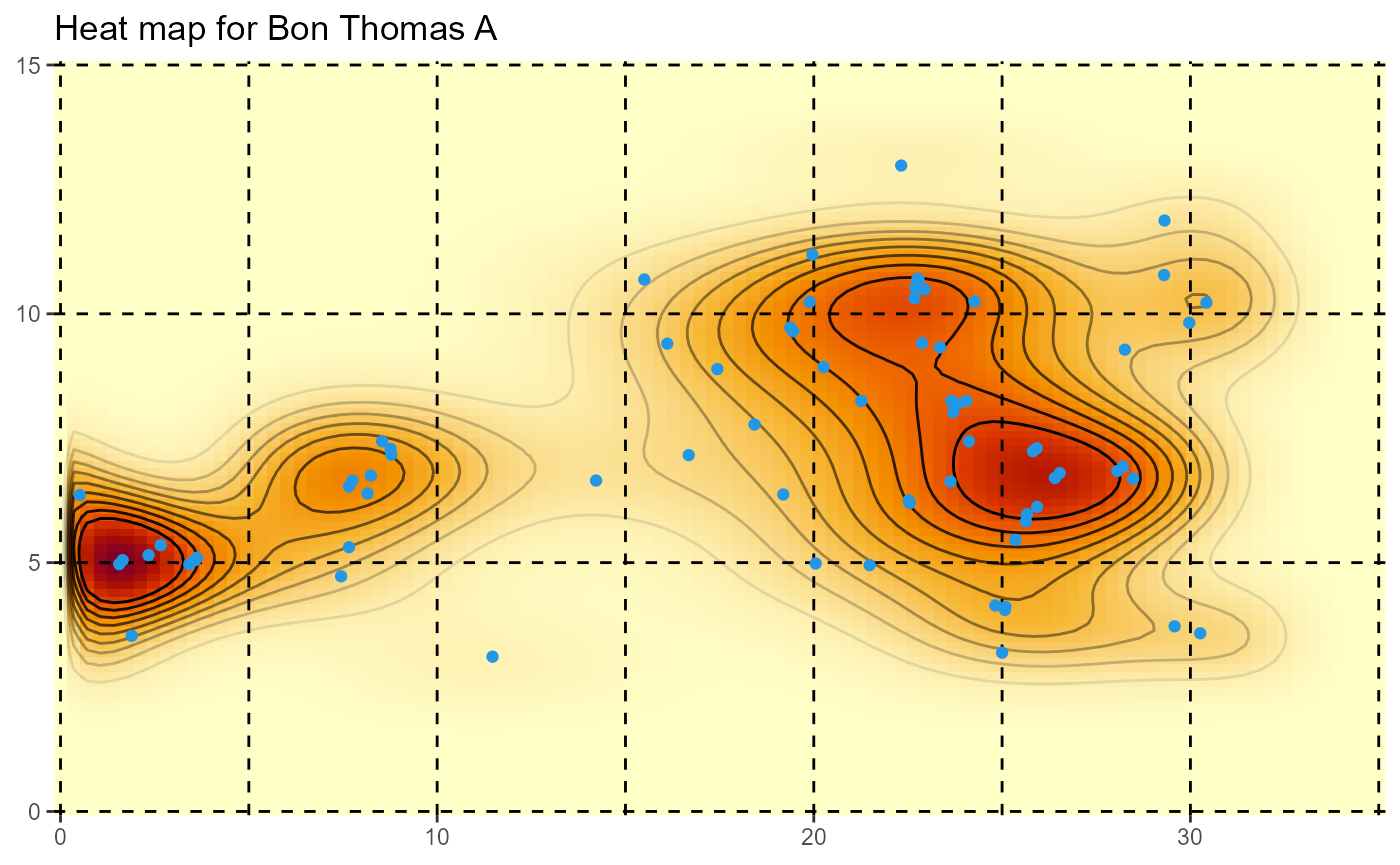

For the State-wide evaluation data, the locations are actually the mid-points of 1m by 1m quadrats, and the weights are the corresponding number of plants in the quadrats. The area of the plotted points is also proprtional to the number of plants.

HeatMap(Site22[,2:3], weights=Site22$NUMPimelea,xrange=c(10,291), yrange=c(1,19), gridsep=10,title="Heat map for Site 22")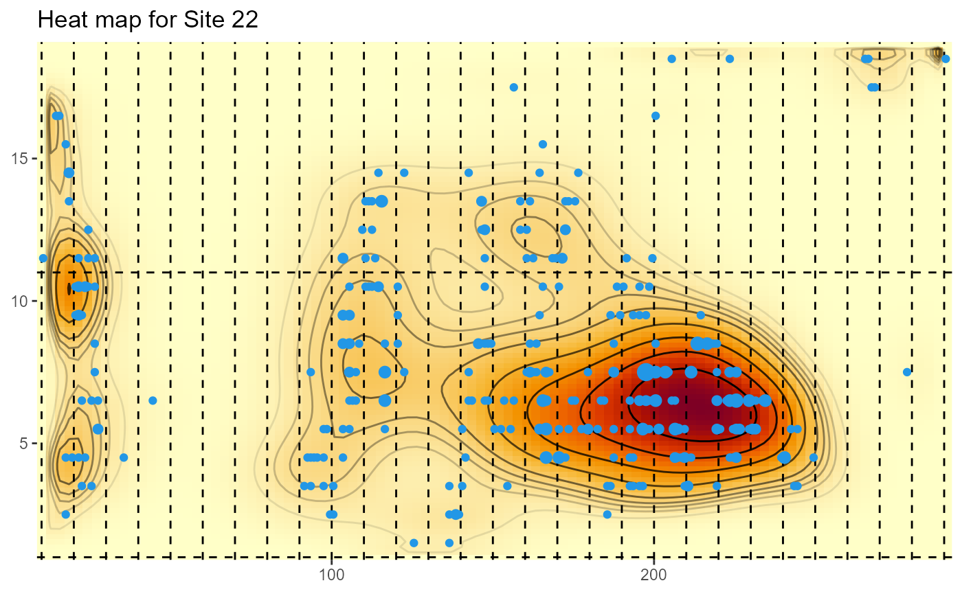

HeatMap(Site29[,2:3], weights=Site29$NUMPimelea,xrange=c(11,25), yrange=c(0,11), gridsep=5,title="Heat map for Site 29")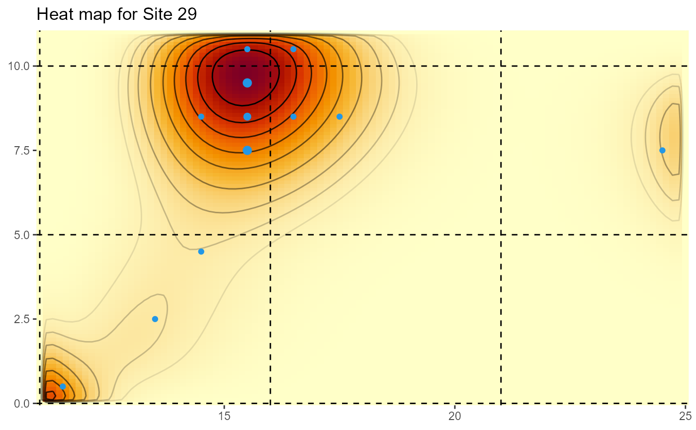

HeatMap(Site45[,2:3], weights=Site45$NUMPimelea,xrange=c(11,86), yrange=c(11,263), gridsep=20,title="Heat map for Site 45")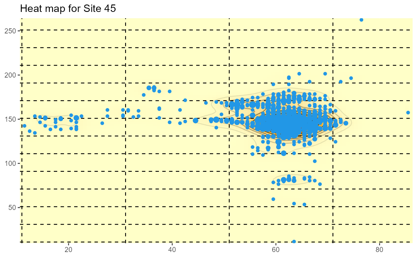

Quadrat Probabilities

Quadrat probabilities can be calculated using the quadratprobs() function. Required inputs are the locations of plants, the lower left coordinate of the grid, with default (0,0), the size of the quadrats, and the minimum grid values, and the maximum grid values. In the example below, it is not necessary to specify the quadratstart argument aswith 5m by 5m quadrats, 5 divides 35 and 15 evenly.

qprobs5 <- quadratprobs(AllPlantsby2020[,2:3], quadratstart=c(0,0),quadratsize=5,
                       xmin=c(0,0),xmax=c(35,15) )
knitr::kable(qprobs5, digits=3)

	[0,5)	[5,10)	[10,15)	[15,20)	[20,25)	[25,30)	[30,35)
[10,15)	0.000	0.000	0.008	0.036	0.067	0.041	0.019
[5,10)	0.067	0.080	0.047	0.087	0.172	0.153	0.026
[0,5)	0.056	0.021	0.011	0.010	0.036	0.045	0.015

On the other hand, for 4m by 4m quadrats, it is useful to be able to specify the quadratstart argument. Note that only internal quadrats are included in the output of quadratprobs().

qprobs4 <- quadratprobs(AllPlantsby2020[,2:3], quadratstart=c(2,1),quadratsize=4,
                       xmin=c(0,0),xmax=c(35,15) )
knitr::kable(qprobs4, digits=3)

	[2,6)	[6,10)	[10,14)	[14,18)	[18,22)	[22,26)	[26,30)	[30,34)
[9,13)	0.000	0.001	0.008	0.033	0.071	0.076	0.046	0.027
[5,9)	0.051	0.065	0.033	0.039	0.076	0.123	0.098	0.018
[1,5)	0.034	0.016	0.010	0.006	0.015	0.037	0.034	0.015

Inclusion Probabilities

Once the quadrat probabilities are calculated, the inclusionprobs() function can calculate the inclusion probabilities. The following gives the inclusion probabilities for various sample sizes. The quadrats are ordered by column of the quadrat probabilities matrix with the top-left quadrat labelled q1.

incprobs <- inclusionprobs(qprobs5,nsim=10000)
knitr::kable(incprobs, digits=3)

ss	q1	q2	q3	q4	q5	q6	q7	q8	q9	q10	q11	q12	q13	q14	q15	q16	q17	q18	q19	q20	q21
1	0.0000	0.0673	0.0580	0.0001	0.0775	0.0190	0.0095	0.0497	0.0122	0.0342	0.0828	0.0091	0.0716	0.1667	0.0358	0.0449	0.1570	0.0451	0.0199	0.0255	0.0141
2	0.0000	0.1333	0.1199	0.0002	0.1602	0.0411	0.0171	0.1020	0.0252	0.0765	0.1654	0.0198	0.1398	0.3282	0.0742	0.0867	0.2971	0.0935	0.0403	0.0505	0.0290
3	0.0000	0.2051	0.1812	0.0006	0.2419	0.0658	0.0250	0.1527	0.0384	0.1196	0.2588	0.0327	0.2107	0.4685	0.1165	0.1290	0.4223	0.1406	0.0632	0.0791	0.0483
4	0.0001	0.2785	0.2398	0.0022	0.3274	0.0922	0.0330	0.2067	0.0513	0.1674	0.3470	0.0452	0.2834	0.5853	0.1599	0.1785	0.5421	0.1914	0.0878	0.1130	0.0678
5	0.0001	0.3490	0.3053	0.0027	0.4119	0.1198	0.0458	0.2654	0.0674	0.2128	0.4381	0.0596	0.3561	0.6831	0.2048	0.2333	0.6422	0.2480	0.1176	0.1468	0.0902
6	0.0001	0.4272	0.3747	0.0033	0.4872	0.1522	0.0580	0.3238	0.0863	0.2625	0.5222	0.0758	0.4289	0.7653	0.2526	0.2905	0.7327	0.3071	0.1488	0.1841	0.1167
7	0.0001	0.5054	0.4404	0.0038	0.5672	0.1845	0.0722	0.3866	0.1063	0.3137	0.6007	0.0929	0.5093	0.8340	0.3060	0.3493	0.8048	0.3691	0.1838	0.2253	0.1446
8	0.0001	0.5855	0.5081	0.0045	0.6435	0.2243	0.0902	0.4564	0.1297	0.3705	0.6749	0.1111	0.5838	0.8839	0.3655	0.4091	0.8584	0.4329	0.2234	0.2705	0.1737
9	0.0001	0.6588	0.5758	0.0052	0.7184	0.2680	0.1078	0.5251	0.1541	0.4362	0.7411	0.1356	0.6553	0.9245	0.4282	0.4725	0.9051	0.5024	0.2593	0.3175	0.2090
10	0.0001	0.7278	0.6517	0.0065	0.7809	0.3168	0.1315	0.5887	0.1818	0.4995	0.8040	0.1607	0.7206	0.9522	0.4970	0.5410	0.9385	0.5757	0.3080	0.3718	0.2452
11	0.0001	0.7868	0.7203	0.0077	0.8375	0.3685	0.1565	0.6619	0.2164	0.5667	0.8582	0.1882	0.7859	0.9713	0.5652	0.6128	0.9637	0.6476	0.3642	0.4316	0.2889
12	0.0002	0.8423	0.7837	0.0089	0.8876	0.4271	0.1884	0.7297	0.2557	0.6398	0.9039	0.2210	0.8446	0.9845	0.6404	0.6850	0.9817	0.7186	0.4210	0.4985	0.3374
13	0.0002	0.8951	0.8448	0.0113	0.9286	0.4969	0.2252	0.7953	0.3045	0.7119	0.9412	0.2632	0.8959	0.9919	0.7093	0.7580	0.9899	0.7857	0.4868	0.5730	0.3913
14	0.0002	0.9355	0.8976	0.0142	0.9570	0.5735	0.2697	0.8599	0.3669	0.7859	0.9656	0.3129	0.9360	0.9958	0.7859	0.8276	0.9962	0.8506	0.5586	0.6541	0.4563
15	0.0002	0.9652	0.9382	0.0170	0.9790	0.6633	0.3262	0.9128	0.4446	0.8536	0.9847	0.3808	0.9648	0.9986	0.8555	0.8890	0.9985	0.9063	0.6452	0.7376	0.5389
16	0.0004	0.9848	0.9695	0.0223	0.9917	0.7566	0.4061	0.9531	0.5372	0.9148	0.9939	0.4702	0.9823	0.9997	0.9159	0.9417	0.9995	0.9491	0.7422	0.8231	0.6459
17	0.0005	0.9957	0.9883	0.0284	0.9974	0.8575	0.5172	0.9810	0.6631	0.9589	0.9987	0.5888	0.9951	1.0000	0.9574	0.9770	0.9999	0.9785	0.8460	0.9051	0.7655
18	0.0009	0.9985	0.9971	0.0419	0.9997	0.9468	0.6850	0.9937	0.8218	0.9894	0.9996	0.7574	0.9988	1.0000	0.9866	0.9937	1.0000	0.9950	0.9369	0.9660	0.8912
19	0.0013	0.9999	1.0000	0.0707	1.0000	0.9974	0.9752	0.9999	0.9872	0.9994	1.0000	0.9812	1.0000	1.0000	0.9998	0.9999	1.0000	0.9999	0.9957	0.9988	0.9937
20	0.0080	1.0000	1.0000	0.9920	1.0000	1.0000	1.0000	1.0000	1.0000	1.0000	1.0000	1.0000	1.0000	1.0000	1.0000	1.0000	1.0000	1.0000	1.0000	1.0000	1.0000
21	1.0000	1.0000	1.0000	1.0000	1.0000	1.0000	1.0000	1.0000	1.0000	1.0000	1.0000	1.0000	1.0000	1.0000	1.0000	1.0000	1.0000	1.0000	1.0000	1.0000	1.0000

Number of Plants Alive at a particular year

(NumberAliveBonThomasA2020 <- NumberAlive(BonThomasA, 2020))
#> Alive 
#>    66

Quadrat Counts of Changes

Change(BonThomasA,2021, quadratsize=5)
#>          x
#> y         [0,5) [5,10) [10,15) [15,20) [20,25) [25,30) [30,35]
#>   [10,15]     0      0       0       0       1       0       0
#>   [5,10)     -1      0       0       0       1       0       0
#>   [0,5)       1      0       0       0      -1       0       0

Change(BonThomasA,2021, quadratsize=4, quadratstart = c(2,1))
#> Warning: 2 points were rejected as lying outside the specified window
#>         x
#> y        [2,6) [6,10) [10,14) [14,18) [18,22) [22,26) [26,30) [30,34]
#>   [9,13]     0      0       0       0       0       0       0       0
#>   [5,9)     -1      0       0       0       0       1       0       0
#>   [1,5)      0      0       0       0      -1       0       0       0

Estimated Total

The EstimatedTotal() command gives the mean, standard deviation, and coefficient of variation (%) for a specified sample size.

EstimatedTotal(BonThomasA, 2021, ss=5, probs=qprobs5, incprobs=incprobs[5,-1]) 
#> [[1]]
#>    Alive 
#> 66.94107 
#> 
#> [[2]]
#> [1] 3.33128
#> 
#> [[3]]
#> Alive 
#>  4.98

EstimatedTotal(BonThomasA, 2021, ss=10, probs=qprobs5, incprobs=incprobs[10,-1]) 
#> [[1]]
#>    Alive 
#> 67.00685 
#> 
#> [[2]]
#> [1] 1.587954
#> 
#> [[3]]
#> Alive 
#>  2.37

EstimatedTotal(BonThomasA, 2021, ss=15, probs=qprobs5, incprobs=incprobs[15,-1]) 
#> [[1]]
#>    Alive 
#> 67.00507 
#> 
#> [[2]]
#> [1] 0.5580785
#> 
#> [[3]]
#> Alive 
#>  0.83